SVM Revisit

By Z.H. Fu https://fuzihaofzh.github.io/blog/

SVM (Support Vector Machine) is an important tool in pattern recognition before the wave of different kind of neural networks. In this post, we revisit the derivation of SVM and get some important intuition of the result.

The original problem

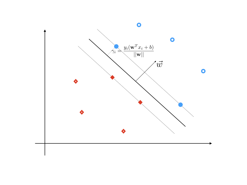
Suppose we have some training data $\mathcal{D}=\{(\mathbf{x}_1, y_1),(\mathbf{x}_2, y_2),\cdots,(\mathbf{x}_n, y_n)\}$, in which $\mathbf{x}$ is a feature vector, and $y_i$ is the class label for each sample and it is -1 or 1. Our task is to find a classifier that uses a separate hyper plane to divide the points in $\mathcal{D}$ into two parts. Points on each side of the hyper plane have the same class label y respectively. This classifier is denoted as $f(\mathbf{x})=\text{sign}(\mathbf{w}^T\mathbf{x}+b)$. For any hyper plane that successfully divide the two classes. We define the geometry margin of the $i$th point as the distance from the point to the hyper plane:

$$\gamma_i=\frac{y_i(\mathbf{w}^Tx_i+b)}{||\mathbf{w}||}$$

We observe that for both classes $y=1$ and $y=-1$, the geometry margin is larger than 0. We can define the geometry margin of our dataset $\mathcal{D}$ as:

$$\gamma=\min_{i=1,\cdots,n} \gamma_i$$

We can see that there are a lot of possible hyper planes. Our ultimate goal is to find the best hyper plane (with parameter $(\mathbf{w}^*,b^*)$) that maximize the geometry margin of the dataset $\mathcal{D}$. Only the geometry margin of the dataset is maximized, can some points between two classes been classified correctly. We can write our problem in the standard optimization form as:

$$\begin{aligned} (P)\ \ \ \ \ \ \ \ \ \ \ \ \ \ \ &\max_{\mathbf{w},b} \gamma\\ s.t.\ & \frac{y_i(\mathbf{w}^T\mathbf{x_i}+b)}{||\mathbf{w}||} \ge \gamma,i \in [1, n] \end{aligned}$$

Convert the original problem into its dual form

To make our problem easy to solve, we can convert it into its dual form. First of all, we define the function margin to help our further derivations. A function margin of $i$th point is defined as:

$$\hat{\gamma_i}=y_i(\mathbf{w}^T\mathbf{x}+b)$$

The function margin of the whole dataset is defined as:

$$\hat\gamma=\min_{i=1,\cdots,n} \hat\gamma_i$$

It can be easily observed that $\gamma=\frac{\hat\gamma}{||\mathbf{w}||}$.
The original problem can be rewritten as:

$$\begin{aligned} &\max_{w,b} \frac{\hat\gamma}{||\mathbf{w}||}\\ s.t.\ & y_i(\mathbf{w}^T\mathbf{x_i}+b) \ge \hat\gamma,i \in [1, n] \end{aligned}$$

We observed that $\hat\gamma$ can be assigned to any value, because if we change $\hat\gamma$ to $\lambda\hat\gamma$, we can adjust ($w$, $b$) to ($\lambda \mathbf{w}$, $\lambda b$) to make the problem unchanged. As a result, we can assign $\hat\gamma=1$ to simplify the problem, i.e.

$$\begin{aligned} &\max_{\mathbf{w},b} \frac{1}{||\mathbf{w}||}\\ s.t.\ & y_i(\mathbf{w}^T\mathbf{x_i}+b) \ge 1,i \in [1, n] \end{aligned}$$

To maximize $ \frac{1}{||\mathbf{w}||}$ is the same as minimize $||\mathbf{w}||$, and the problem changes to:

$$\begin{aligned} &\min_{\mathbf{w},b} \frac{1}{2}||\mathbf{w}||^2\\ s.t.\ & y_i(\mathbf{w}^T\mathbf{x_i}+b) \ge 1,i \in [1, n] \end{aligned}$$

Next, we want to merge the constrains into the objective function to make it an unconstrained problem. We want to design a function $g_i(\mathbf{w},b)$, s.t.

$$g_i(\mathbf{w},b)=\left\{ \begin{aligned} 0&\ \ \ \text{if } (\mathbf{w},b) \text{ fulfill the ith constrain}\\ \infty&\ \ \ \text{otherwise} \end{aligned} \right.$$

It can be written into a more compact form with the $\max$ notation:

$$g_i(\mathbf{w},b)=\max_{\alpha_i\ge0}\alpha_i[1-y_i(\mathbf{w}^T\mathbf{x}+b)]$$

In which, $\alpha_i$ is called the Largrange multiplier. If $(\mathbf{w},b)$ fulfill the constrain, $1-y_i(\mathbf{w}^T\mathbf{x}+b)\le0$ and $\alpha_i=0$ to attain its max value 0. On the other hand, if $(\mathbf{w},b)$ violate the constraint, $1-y_i(\mathbf{w}^T\mathbf{x}+b)>0$ and $\alpha_i=\infty$ to attain its max value $\infty$.
Thus, the optimization problem can be written as $$\begin{aligned}&\min_{\mathbf{w},b}\frac{1}{2}||\mathbf{w}||^2+\sum_{i=1}ng_i(\mathbf{w},b)\
=&\min_{\mathbf{w},b}\frac{1}{2}||\mathbf{w}||^2+\sum_{i=1}n\max_{\alpha_i\ge0}\alpha_i[1-y_i(\mathbf{w}^T\mathbf{x}+b)]\
=&\max_{\alpha_i\ge0}\min_{\mathbf{w},b}\frac{1}{2}||\mathbf{w}||^2+\sum_{i=1}n\alpha_i[1-y_i(\mathbf{w}^T\mathbf{x}+b)]\
=&\max_{\alpha_i\ge0}\min_{\mathbf{w},b}J(\mathbf{w},b,\mathbf{\alpha})
\end{aligned}$$
In which $J(\mathbf{w},b,\mathbf{\alpha})=\frac{1}{2}||\mathbf{w}||^2+\sum_{i=1}^n\alpha_i[1-y_i(\mathbf{w}^T\mathbf{x}+b)]$. The inside minimize problem can be solved by setting the derivative to 0:

$$\begin{aligned} \frac{\partial J(\mathbf{w},b,\mathbf{\alpha})}{\partial \mathbf{w}}&=\mathbf{w}-\sum_{i=1}^n\alpha_iy_i\mathbf{x_i}=0\\ \frac{\partial J(\mathbf{w},b,\mathbf{\alpha})}{\partial \mathbf{b}}&=-\sum_{i=1}^n\alpha_iy_i=0 \end{aligned}$$

We get $\mathbf{w^* }=\sum_{i=1}^n\alpha_iy_i\mathbf{x_i}$, substitute it into the optimization problem we get:

$$\max_{\alpha_i\ge0}\sum_{i=1}^n\alpha_i-\frac{1}{2}\sum_{i=1}^n\sum_{j=1}^ny_iy_j\alpha_i\alpha_j\mathbf{x_i}^T\mathbf{x_j}$$

We write it into a formal optimization problem:

$$\begin{aligned} (D)\ \ \ \ \ \ \ \ \ \ \ \ \ \ \ \min_{\alpha}\ \ & \frac{1}{2}\sum_{i=1}^n\sum_{j=1}^ny_iy_j\alpha_i\alpha_j\mathbf{x_i}^T\mathbf{x_j}-\sum_{i=1}^n\alpha_i \\ s.t. \ \ &\sum_{i=1}^n\alpha_iy_i=0\\ &\alpha_i\ge0, i \in [1,n] \end{aligned}$$

This is the dual optimization problem of problem (P) and it is a standard Quadratic Programming which can be solved by a lot of solvers.

Some obervations and intuitions

1. The variable of the primal optimization problem (P) is to optimize $(\mathbf{w},b)$ while the dual problem (D) is to optimize the dual variable $\mathbf{\alpha}$. The length of dual variable equals to the number of constrains of the primal problem.

2. If $\alpha_i=0$, $y_i(\mathbf{w}^T\mathbf{x_i}+b)>1$ the function margin of this is not equal to the function margin of the dataset ($\hat\gamma=1$) . It means that the margin of this sample is not the smallest among others.
   If $\alpha_i>0$, it means that the $i$th constrain is active and $y_i(\mathbf{w}^T\mathbf{x_i}+b)=1$. The function margin of the $i$th sample equals to the function margin of the dataset. This sample is called a support vector.

3. We observe the optimal value of $\mathbf{w^*}$:

$$\mathbf{w}^*=\sum_{i=1}^n\alpha_iy_i\mathbf{x}$$

In which $\alpha_i=0$ for all non support vectors, which means that the value of $\mathbf{w^*}$ is only determined by support vectors.

Reference

[1] 李航. 统计学习方法.

[2] Xiaogang, Wang. “ENGG5202 Lecture notes.” Chapter8.